AlanLichty
Moderator
This borders on a Once Upon a Time tale but in the early 1980's we weren't using the term Digital Imaging to describe computer graphics. There were quite a number of folks working in the field of computer graphics but the notion of a hand held digital camera was a pipe dream at best. I think about how much things have changed every time I grab a slider in Lightroom or Photoshop to edit an image. These were not the Good Old Days(TM).
I was hired by the Utah Archaeological Center to facilitate computing tasks in the late 1970's after funding for Middle East work dried up. One of the early projects was to develop methods of using remote sensing data for predictive models of archaeological site locations primary based on Landsat data. Landsat 3 was the primary data set we used which did actually use CCD (Charge Coupled Device) sensors similar to our modern camera sensors but were rather cumbersome with profoundly limited resolution. Landsat scenes were purchased from NASA on 9 track tapes and the ground resolution was roughly 75 meters.
Through grant funding the University of Utah Anthropology department gave me the task of building a computational facility capable of allowing the department faculty to utilize computer graphics in their research. This is a set of photos of that facility and some of the output we generated. Absolutely everything that was generated was homegrown FORTRAN software I wrote back then with the exception of a set of modules we got from NASA to perform analysis on the Landsat data.
What did it take to process computer graphics? In our case I bought a DEC VAX 11/730 computer, a Kennedy 4500 9-track tape drive, a Ramtek graphics processor and monitor, and a Matrix Instruments camera system to capture the output. Total cost for the hardware came in at around $60,000.
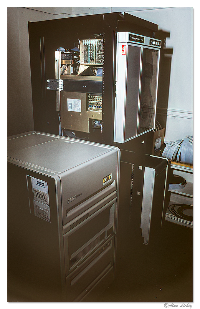
The graphics processor is between the tape drive and the tapes. The graphics system also included a color monitor that could display a 1280x1024 image (yup - just short of a one megapixel screen). We also added a 60" Summagraphics digitizing table so we could build maps and record areas that had been surveyed off of USGS Quad sheets.
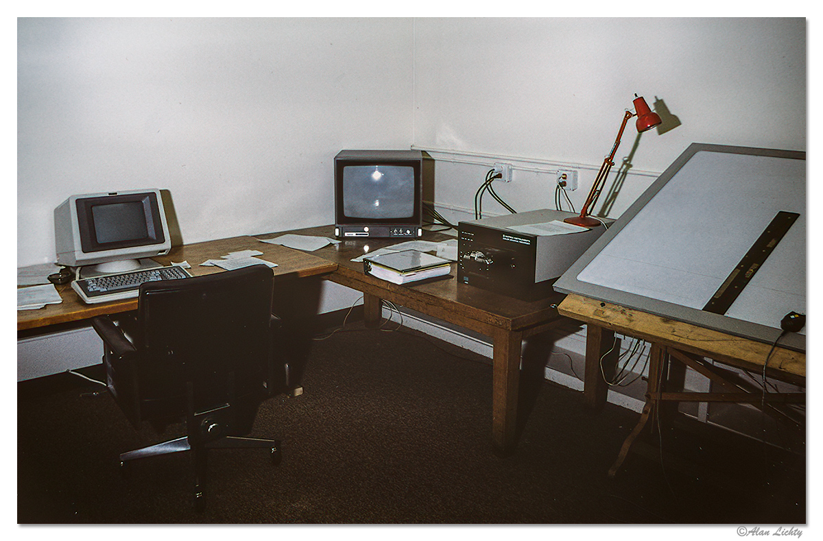
The monitor is in the center and the camera system is just to the right of that. The camera system had a small version of the 1280x1024 monitor that displayed images in black and white and had a color wheel so we could get color output by taking a triple exposure with the red, green, and blue parts of the color wheel. I went through a lot of rolls of film getting the triple exposure values calibrated. The attached camera was an Olympus SLR with a fixed focus lens that was calibrated for the small internal monitor. The camera system was custom built to allow it to synchronize with the Ramtek graphics system.
Computing power was the biggest obstacle - sampling a Landsat scene could take hours of CPU time which I had to do on one of the larger campus computers as our little VAX wasn't up to that kind of number crunching with only 2MB of RAM.
Examples of what kinds of images we were able to produce as graphics output - I used a FORTRAN subroutine library (Plot79) developed by the Univ of Utah Math department to create vector based graphics and developed a series of programs that allowed our faculty to digitize maps for lectures and publications both for archaeology as well as biological anthropology. All of the output examples shown below are 1 megapixel images.
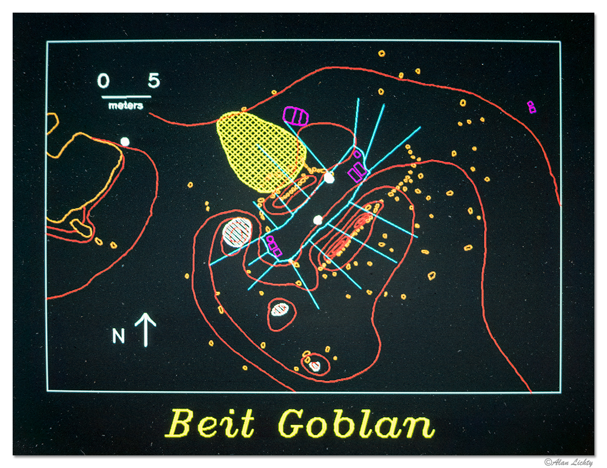
This first image was a map of a living bedouin black tent encampment in Petra showing the outlines of the tent living area (light blue) and the distribution of trash and belongings. The intent here was to record an example of how a tent site is used as a model for how to interpret artifact distributions in archaeological sites. Note that the living area itself is the clean spot inside of the tent outline.
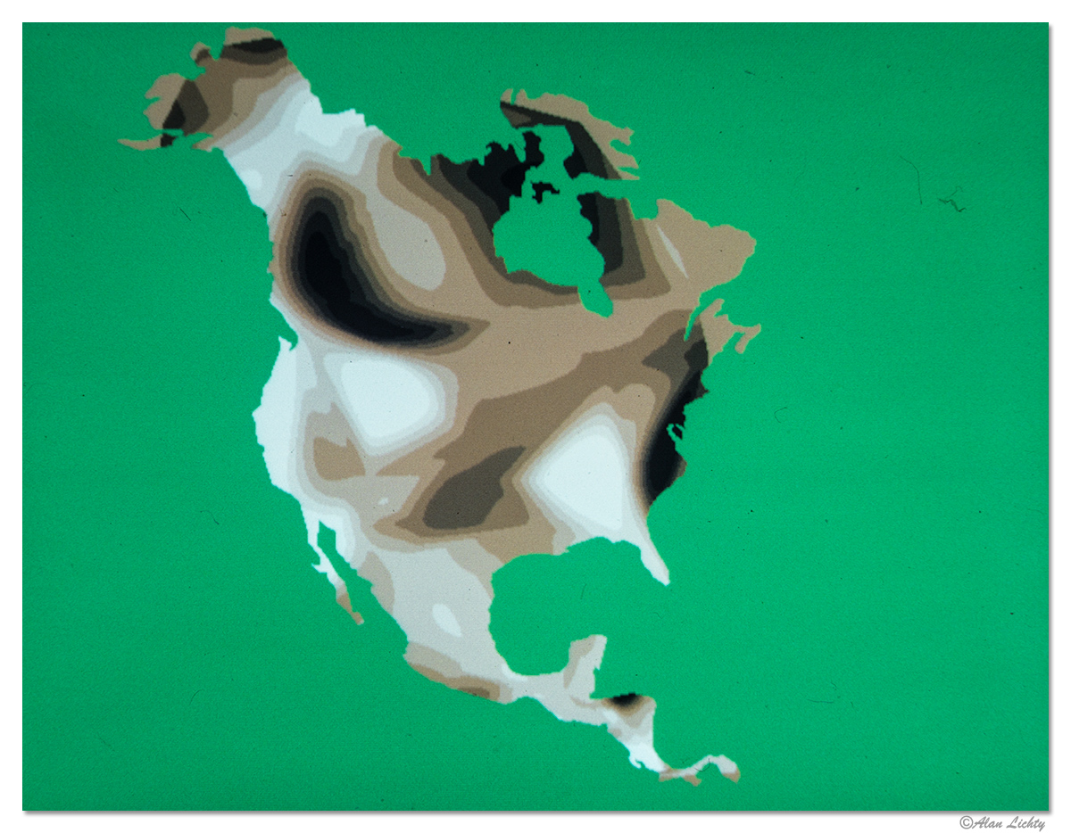
The next one shows blood haptoglobin genetic samples for North American Indian tribes with the mask of a North America map for locational orientation. This was done entirely in custom FORTRAN code. Things I can do in minutes in Photoshop these days took days of coding back in the mid 80's.
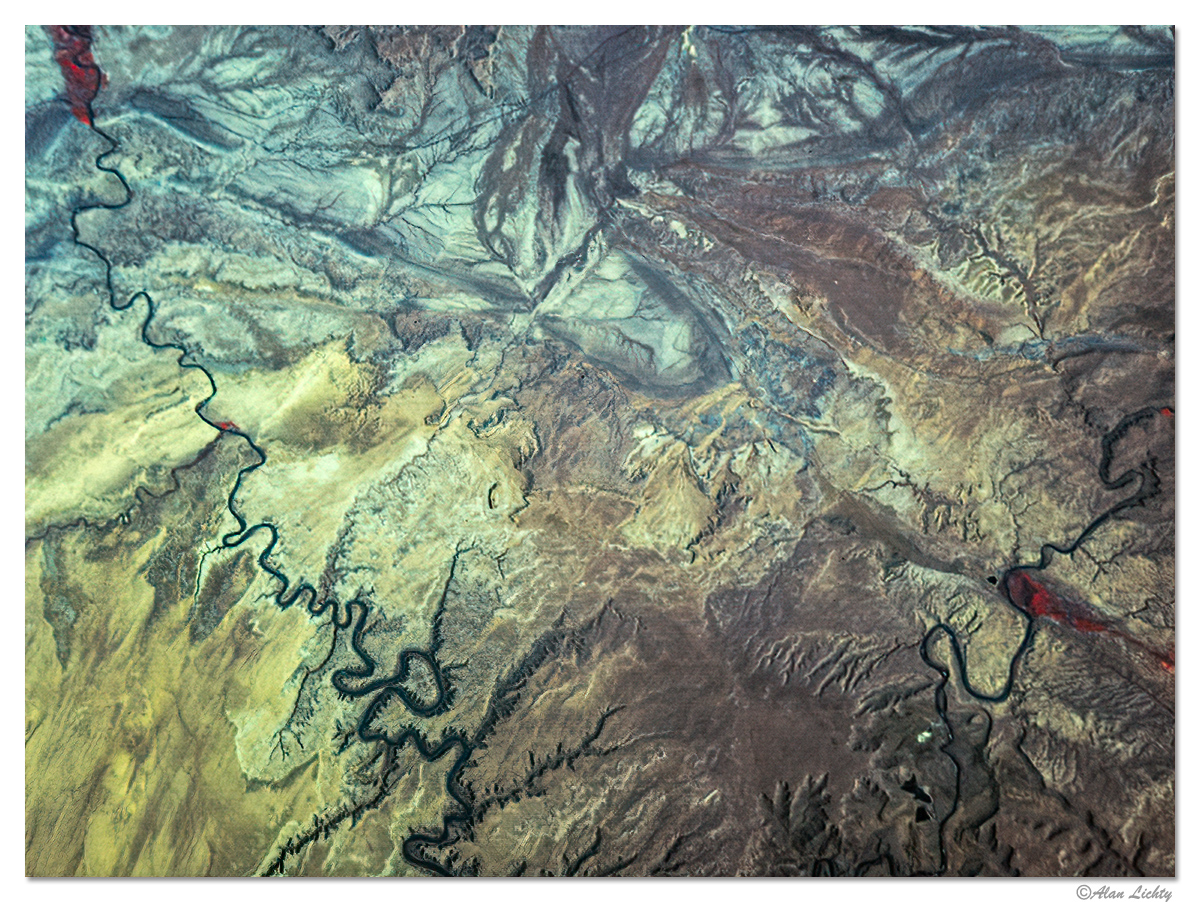
I loaded up a portion of a Landsat scene so I could try my hand at false color composites because I thought satellite images were seriously cool. The part that gets rather convoluted - this takes digital output from a satellite which is processed in our computers so we could display it on a screen and then take an analog photo of the image on slide film so I could turn around and scan it into a digital image to show you here
This is a scene in southern Utah with the Green River area in the upper left and Moab down in the lower right. I-70 is visible heading east out of the Green River area at the top. The false color composites typically used the IR band so vegetated areas show up in red.
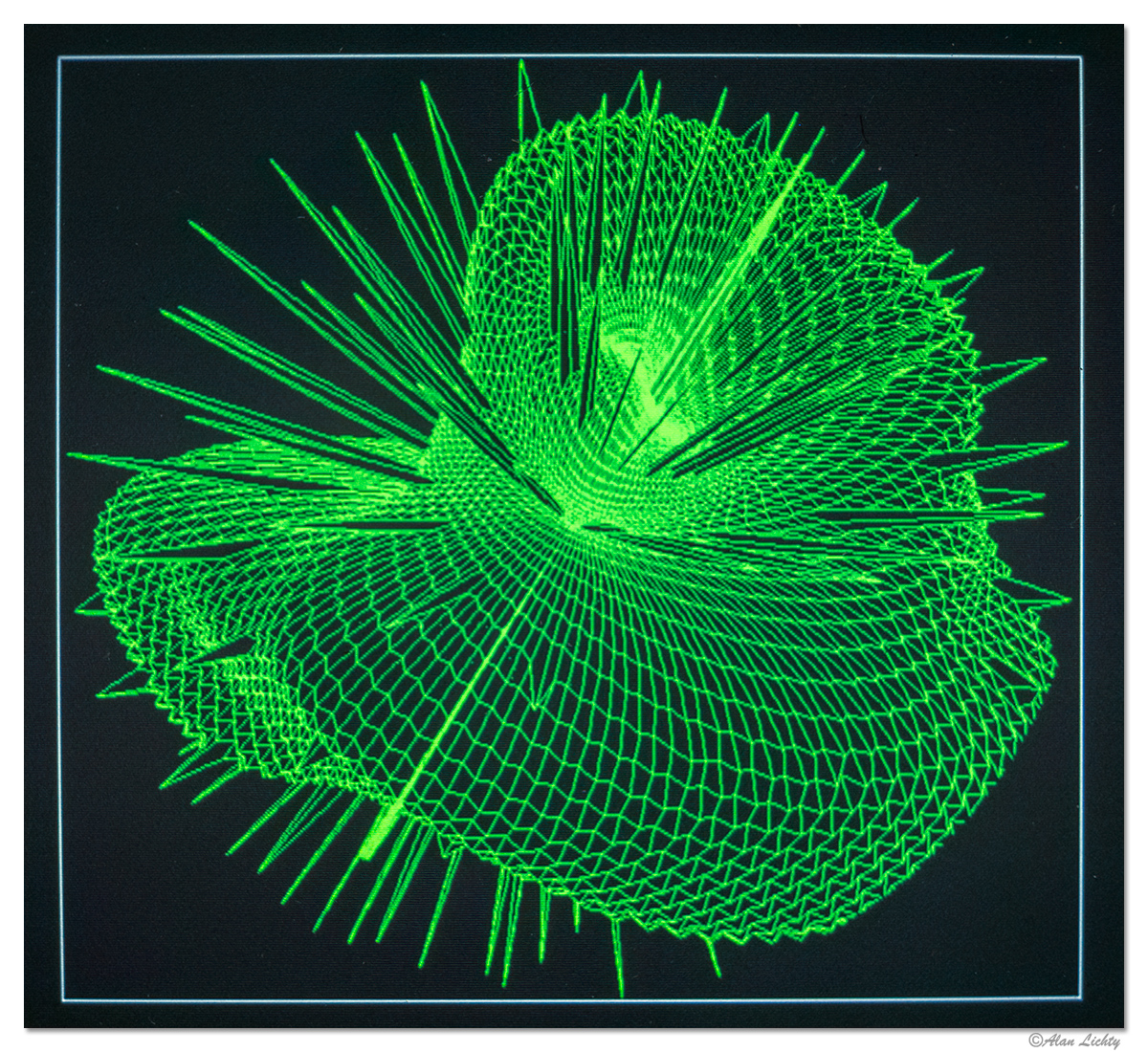
For the math geeks I also have a copy of the output from one of the demos in the Plot79 subroutine library - in this case a mathematical function mapped onto polar coordinates:
Thanks if you stuck around to the end of this
I was hired by the Utah Archaeological Center to facilitate computing tasks in the late 1970's after funding for Middle East work dried up. One of the early projects was to develop methods of using remote sensing data for predictive models of archaeological site locations primary based on Landsat data. Landsat 3 was the primary data set we used which did actually use CCD (Charge Coupled Device) sensors similar to our modern camera sensors but were rather cumbersome with profoundly limited resolution. Landsat scenes were purchased from NASA on 9 track tapes and the ground resolution was roughly 75 meters.
Through grant funding the University of Utah Anthropology department gave me the task of building a computational facility capable of allowing the department faculty to utilize computer graphics in their research. This is a set of photos of that facility and some of the output we generated. Absolutely everything that was generated was homegrown FORTRAN software I wrote back then with the exception of a set of modules we got from NASA to perform analysis on the Landsat data.
What did it take to process computer graphics? In our case I bought a DEC VAX 11/730 computer, a Kennedy 4500 9-track tape drive, a Ramtek graphics processor and monitor, and a Matrix Instruments camera system to capture the output. Total cost for the hardware came in at around $60,000.
The graphics processor is between the tape drive and the tapes. The graphics system also included a color monitor that could display a 1280x1024 image (yup - just short of a one megapixel screen). We also added a 60" Summagraphics digitizing table so we could build maps and record areas that had been surveyed off of USGS Quad sheets.
The monitor is in the center and the camera system is just to the right of that. The camera system had a small version of the 1280x1024 monitor that displayed images in black and white and had a color wheel so we could get color output by taking a triple exposure with the red, green, and blue parts of the color wheel. I went through a lot of rolls of film getting the triple exposure values calibrated. The attached camera was an Olympus SLR with a fixed focus lens that was calibrated for the small internal monitor. The camera system was custom built to allow it to synchronize with the Ramtek graphics system.
Computing power was the biggest obstacle - sampling a Landsat scene could take hours of CPU time which I had to do on one of the larger campus computers as our little VAX wasn't up to that kind of number crunching with only 2MB of RAM.
Examples of what kinds of images we were able to produce as graphics output - I used a FORTRAN subroutine library (Plot79) developed by the Univ of Utah Math department to create vector based graphics and developed a series of programs that allowed our faculty to digitize maps for lectures and publications both for archaeology as well as biological anthropology. All of the output examples shown below are 1 megapixel images.
This first image was a map of a living bedouin black tent encampment in Petra showing the outlines of the tent living area (light blue) and the distribution of trash and belongings. The intent here was to record an example of how a tent site is used as a model for how to interpret artifact distributions in archaeological sites. Note that the living area itself is the clean spot inside of the tent outline.
The next one shows blood haptoglobin genetic samples for North American Indian tribes with the mask of a North America map for locational orientation. This was done entirely in custom FORTRAN code. Things I can do in minutes in Photoshop these days took days of coding back in the mid 80's.
I loaded up a portion of a Landsat scene so I could try my hand at false color composites because I thought satellite images were seriously cool. The part that gets rather convoluted - this takes digital output from a satellite which is processed in our computers so we could display it on a screen and then take an analog photo of the image on slide film so I could turn around and scan it into a digital image to show you here
This is a scene in southern Utah with the Green River area in the upper left and Moab down in the lower right. I-70 is visible heading east out of the Green River area at the top. The false color composites typically used the IR band so vegetated areas show up in red.
For the math geeks I also have a copy of the output from one of the demos in the Plot79 subroutine library - in this case a mathematical function mapped onto polar coordinates:
Thanks if you stuck around to the end of this